Noise figure measurements with a spectrum analyzer and a noise source

Noise figure is an important property of RF and microwave building blocks such as amplifiers, but can be challenging to measure without specialized equipment. However, if a calibrated broadband noise source is available, an ordinary spectrum analyzer is almost enough to accurately measure noise figure if some care is taken. Just about the right thing to do while waiting for parts during the 2021—2023(?) global component shortage, which has put all my other projects on hold.

The Y-factor method

There are several ways of measuring noise figure, but one of the most basic ways is the Y-factor method. Recall that, according to Planck's radiation law, a resistor $R$ at temperature $T$ produces a RMS noise voltage \[V_{\rm n}=\sqrt{\frac{4hfBR}{\mathord{\rm e}^{hf/kT}-1}}\] in a bandwidth $B$ centered at frequency $f$, where $k$ is Boltzmann's constant, and $h$ is Planck's constant. At low frequencies, when $hf\ll kT$, this can be approximated by $V_{\rm n}=\sqrt{4kTBR}.$ Thus, when a matched resistor at temperature $T$ is connected to the device under test (DUT), it delivers a noise power of $N=kTB$ to its input. If the DUT has gain $G$, and the resistor temperature is once left at room temperature $T_1$, and once brought to a higher temperature $T_2$, the noise power at the DUT output in each case is \[\begin{align*} N_1&=GkT_1B+N_\text{added},\\ N_2&=GkT_2B+N_\text{added}, \end{align*}\] where $N_\text{added}$ is the noise added by the DUT, which is the quantity we are interested in. This noise can be expressed in terms of an equivalent temperature $T_{\rm e}$, i.e., $N_\text{added}=GkT_{\rm e}B$. Solving the above equations for $T_{\rm e}$ yields \[T_{\rm e}=\frac{T_1-YT_2}{Y-1},\] where \[Y=\frac{N_1}{N_2}\] is called the Y-factor. Hence by measuring $N_1$ (resistor at room temperature $T_1$) and $N_2$ (resistor at elevated temperature $T_2$), we can work out $T_{\rm e}$.

Usually the DUT noise is specified in terms of noise figure, which is defined as the quotient of the signal-to-noise-ratios at the DUT input and output, assuming the input noise power is $N_{\rm i}=kT_0B$, with temperature $T_0$ mostly taken to be 290 K. By substituting from above and simplifying we find \[F=\frac{S_{\rm i}/N_{\rm i}}{S_{\rm o}/N_{\rm o}}=\frac{S_{\rm i}/(kT_0B)}{GS_{\rm i}/(Gk(T_0+T_{\rm e})B)}=1+\frac{T_{\rm e}}{T_0}.\] Often $F$ is expressed in dB, i.e., $F({\rm dB})=10\cdot\log F$. Sometimes $F$ in linear units is referred to as noise factor, and only $F({\rm dB})$ is called noise figure.

Since it is impractical to bring a matched resistor at the DUT input to a high enough temperature so that $Y$ is sufficiently different from one, semiconductor noise sources are used, which can be switched on and off, thereby changing their effective noise temperatures between $T_1$ and $T_2$. This is characterized in terms of the excess noise ratio (ENR), often stated in dB, and defined by \[{\rm ENR}({\rm dB})=10\cdot\log\Bigl(\frac{T_2-T_1}{T_1}\Bigr),\] where $T_1$ is usually taken to be 290 K.

Therefore, when a noise source with known ENR is available, and the noise powers $N_1$ and $N_2$ at the DUT output are measured in a bandwidth $B$, centered at frequency $f$, that is small with respect to the DUT bandwidth, the DUT equivalent noise temperature $T_{\rm e}$ and its noise figure $F$ at frequency $f$ can be calculated by substituting from above: \[F=\frac{\rm{ENR}}{Y-1},\] with both ${\rm ENR}$ and $F$ in linear units. (These considerations tacitly assume that the noise power spectral density is constant over $B$.)

So far it was assumed that the system measuring $N_1$ (noise source off or cold) and $N_2$ (noise source on or hot) itself does not contribute any noise. The total noise figure of a series connection of a device with noise figure $F_1$ and gain $G_1$, followed by a device with noise figure $F_2$, is given by Friis' formula as $F_\text{tot}=F_1+(F_2-1)/G_1$. This implies the following procedure to eliminate the system noise contribution:

1. Calibration measurement: The noise source is connected directly (without DUT), and the noise powers $N_1$ and $N_2$ (cold and hot) are measured. Then the measurement system noise figure $F_{\rm cal}={\rm ENR}/(Y_{\rm cal}-1)$ is found, with $Y_{\rm cal}=N_2/N_1$.

2. DUT measurement: With the DUT connected to the noise source, the noise powers $N_1'$ and $N_2'$ (cold and hot) are measured.

3. DUT gain and total noise figure: The DUT gain is found from $G=(N_2'-N_1')/(N_2-N_1)$, and the total noise figure from $F_{\rm tot}={\rm ENR}/(Y_{\rm tot}-1)$, with $Y_{\rm tot}=N_2'/N_1'$.

4. System noise correction: By using Friis' formula, the DUT noise figure is found as $F=F_{\rm tot}-(F_{\rm cal}-1)/G$.

It can be seen from the last equation that for a large gain DUT the system noise correction is less important, whereas it plays a crucial role for devices with small gain or even attenuation. Also, it can be seen that when $F$ is much higher than ${\rm ENR}$, $Y$ becomes very close to unity, making a reliable measurement difficult.

More on noise figure theory and measurement can be found in [1] and [2].

The test setup

I used a Hewlett-Packard model 346B noise source, specified from 10 MHz to 18 GHz, and with 15 dB nominal ENR. The actual ENR measured at some frequency points is printed on the backside of the source. To measure noise power in a specified bandwidth, a Rohde & Schwarz FSIQ26 spectrum analyzer was used. It provides a 10 MHz resolution filter and a RMS detector. Since this unit has no built-in preamplifier, a model LNA-300B low-noise amplifier made by RF-Bay, Inc. was used as a preamplifier at the analyzer input. This amplifier is specified from 40 MHz to 3 GHz and has a noise figure of about 1.3 dB, which significantly lowers the system noise contribution.

Measuring noise figure involves measuring low powers and comparing signal levels differing by only small amounts (cf. the calculation of $Y$ above). For this reason, a well-shielded test setup is absolutely crucial. When cables cannot be avoided, they should be doubly shielded and of high quality. Since noise figure measurements are sensitive to the DUT input matching, only high quality connectors and adapters should be used. Also, fluctuating quantities are being measured, therefore long averaging periods are needed in order to yield smooth traces, which requires a stable test setup.

Data analysis

To calculate noise figure and gain from spectrum analyzer trace data accordig to the method outlined above, I wrote a couple of lines in GNU Octave. They provide a function nfmeas with syntax:

NF_uncorr = nfmeas(enrtable, freq, dut_h, dut_c)
[NF, Gain] = nfmeas(enrtable, freq, dut_h, dut_c, cal_h, cal_c, reftemp, meastemp)

The 2×n matrix enrtable contains in each column a frequency and ENR pair, as printed on the noise source backside. The equal length vectors freq, dut_h, dut_c, cal_h, cal_c contain the respective power measurements at the frequencies in freq. When cal_h and cal_c are specified, the noise figure is corrected for system noise and the DUT gain is provided as an optional return value. Then the ENR reference temperature (usually 290 K) must be specified, and also the actual noise source temperature during measurement, because an additional temperature correction is applied. All ENR and power data, as well as the return values, are in linear units (not in dB).

The function file as well as scripts to run the example measurements shown below are available for download along with the measured data of the examples shown below.

Measuring an attenuator

As explained above, a DUT with attenuation is particularly challenging because the system noise correction is much more significant and can easily dominate the DUT noise, also the signal levels involved are lower. Therefore, I tested the setup with a 3 dB attenuator (Midwest Microwave 18 GHz Model 219 type N). The spectrum analyzer settings for all four measurements were as follows:

• Start: 30 MHz, Stop: 3 GHz
• Resolution bandwidth: 10 MHz
• Video bandwidth: 1 kHz
• RF attenuation: 1 dB
• Detector: RMS
• No. of averages: 250

The stop frequency was dictated by the preamplifier. With a higher bandwidth amplifier, the frequency range could be extended (the 346B noise source is characterized up to 18 GHz). The sweep time for these settings was 760 ms, so one measurement takes a bit over three minutes. As an example, here is a plot of the calibration measurement with noise source on.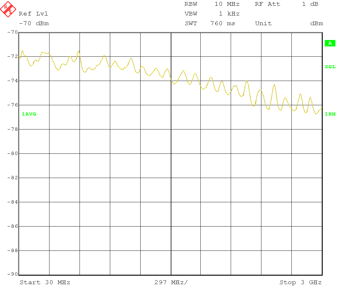

Note that in this plot the indicated power at each frequency point is not the noise power in the noise bandwidth of the resolution filter as seen by the analyzer input, but is actually slightly lower by a constant offset, despite using the RMS detector. This is because of the heavy video filtering (VBW≪RBW), see [3] for more details on absolute noise power measurements with spectrum analyzers. The actual offset depends on the transfer function of the video filter and the noise distribution (for thermal noise a Gaussian amplitude distribution and a Rayleigh envelope distribution), and possibly (depending on the VBW setting) on the RMS averaging and trace averaging. However, this offset is irrelevant here because it drops out when the Y-factor and the gain are calculated.

The results confirm the expectation to see a gain of −3 dB, and a noise figure of +3 dB. There is some amount of ripple on the noise figure and gain traces, and at higher frequencies the noise figure curve shows some residual noise (possibly due to the increasing noise figure of the preamplifier at these frequencies), which could be eliminated by a lager number of averages or possibly by selecting a lower video bandwidth on the spectrum analyzer. Also, the curves could use some post-processing like a smoothing filter. But overall, this result is very satisfactory.

Measuring an amplifier

Next I tested a Mini-Circuits model ZFL-500HLN low noise amplifier. It has a frequency range of 10 MHz to 500 MHz, a gain of 19 dB (min.) with ±0.4 dB flatness, a 1 dB compression point of +16 dBm (output referred), and the nominal noise figure is quoted as 3.8 dB (the “Typical Performance Data/Curves” shown in the datasheet are little a worse). The amplifier was operated from a supply voltage of 15 V.

In this case, the following spectrum analyzer settings were used; they yield a sweep time of about 120 ms, so each measurement takes about 30 s:

• Start: 30 MHz, Stop: 500 MHz
• Resolution bandwidth: 10 MHz
• Video bandwidth: 1 kHz
• RF attenuation: 10 dB
• Detector: RMS
• No. of averages: 250

The resulting traces for noise figure and gain are nice and smooth, indicating that a noise figure measurement of a DUT with gain is much easier. The noise figure is found to be slightly above 4 dB, hence a bit higher than indicated in the datasheet, but it is definitively of the expected order. The typical data in the datasheet shows a very flat gain between 20.66 dB and 20.97 dB for 15 V supply voltage over the entire frequency range, which differs by about 4 dB from what is seen here. The datasheet does not say whether the quoted gain is calculated from S₂₁-data with respect to 50 Ω, or if it is the transducer power gain (the quotient of the actual power delivered to the load and the maximum power available from the source) as measured by this method. These two gain concepts are different for a poorly matched DUT.

For comparison, I measured the S-parameters of the amplifier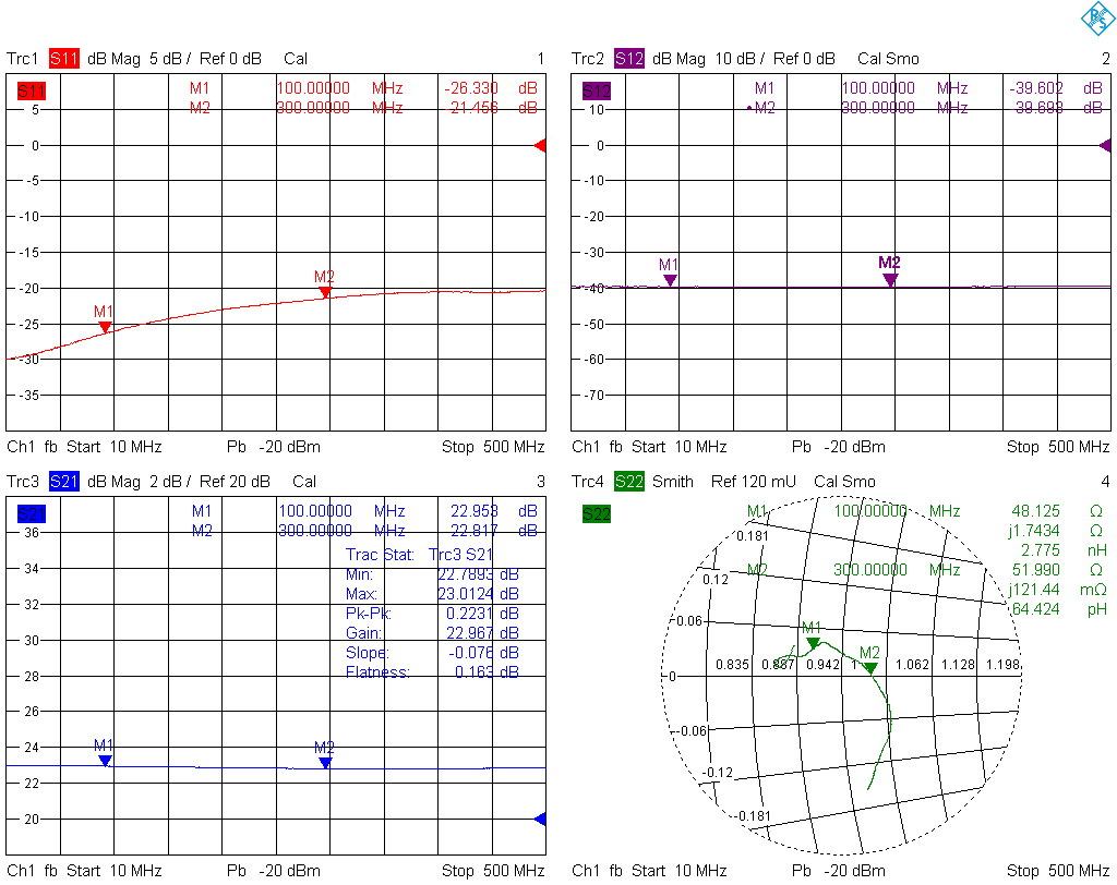. The gain calculated from S₂₁ is about 23 dB, also higher than the datasheet value, but closer to the above measurement. Flatness is excellent: about 0.16 dB, and 0.22 dB peak-to-peak variation. Also, the input matching is quite good for a low-noise amplifier (more than 20 dB return loss).

Bibliography

1. Pozar, D.M.: Microwave Engineering. 4th Ed. New York: Wiley (2012).
2. Keysight Technologies: Fundamentals of RF and Microwave Noise Figure Measurements. Keysight Application Note 5952-8255.
3. Rauscher, C., Janssen, V., Minihold, R.: Fundamentals of Spectrum Analysis. München: Rohde & Schwarz (2001).