Characterizing a SMA calibration kit
Since you are reading this you probably know well that a vector network analyzer (VNA) derives much of its accuracy from the calibration done before every measurement (which should more precisely be called vector error correction). It corrects for systematic errors of the instrument as well as for influences of the particular test setup, e.g., cables, adapters, test fixtures, etc. In most cases, if no port extension, de-embedding or fixture removal is done, calibration also fixes the reference planes of the measurement. To do a calibration one needs a good quality calibration kit. I'm fortunate to own a precise and extremely expensive (depending on configuration and options these easily set you back by a five digit amount) 3.5 mm SOLT (or TOSM in Rohde & Schwarz terms) calibration kit manufactured by Maury Microwave, which is good to 26.5 GHz. However, for everyday situations and at low frequencies (up to 2 GHz, say) the precision of this kit is not always needed, and in order to save wear and tear on it, I wanted to get a cheap sacrificial kit as a supplement.
A cheap alternative
Looking on ebay and AliExpress for an SMA cal kit, one sees several far eastern (i.e., Chinese) kits with varying prices and probably of varying quality. I finally decided to take a look at a very cheap one, which contains open short and load calibration standards in both a male and female version:

This kit was about € 40 on AliExpress including delivery from China to Germany. Apparently similar kits are available from various vendors, and you can find them also on amazon. There are several versions of this kit. In some of them the cal standards have an extremely short body that cannot be held while turning the connector nut, so that the body will rotate. Of course this is not good for your test cables and adapters. It would even be better if the body of the male standards had flats to hold it with a wrench like on professional adapters, but what can you expect for 40 Euros? If I remember correctly, the male standards are rated up to 3 GHz, and the female to 6 GHz. Needless to say the kit comes with no correction data whatsoever.
Metrological precision aside, the first concern with cheap SMA connectors of dubious origin is that they might damage your outrageously expensive 3.5 mm connectors when mating with them, and be it only once for a characterization measurement. Therefore it is a good starting point to look for the following issues: Burrs on the pin of the male connector, pin protrusion/recession (preferably using a connector gauge), overall geometry, and the female center contact. In cheap connectors this is frequently only a sleeve with a single slot which can have sharp edges that cause damage to the center pin of a male connector. Nevertheless, after close inspection I decided that the kit is safe to go, even though the center pin seems to have some slight roughness on its lead-in taper (I would not mate it with slotless PC3.5 mm connectors, however).
Before doing any measurements, it is a good idea to calibrate one's expectations of this kit. There is a reason that professional cal kits do not have SMA connectors, but exclusively air dielectric connectors like PC3.5 mm or K connectors, etc. The SMA connector has a poorly defined geometry due to its PTFE dielectric, especially at the mating surface, which is usually slightly recessed from the mating plane, leaving an air gap between the dielectrics of both connectors. This will entail increased return loss and poor repeatability. And yes, this can already be seen at 1 GHz if you look closely enough with a high quality VNA. Moreover, SMA is not as durable as lab grade air dielectric precision connectors, even though their center conductors are not as delicate as in air dielectric connectors because of the firm stabilization due to the PTFE dielectric. Reputable manufacturers often specify SMA connectors for about only 100 mating cycles, although in practice they should last much longer if not abused. Besides connector precision and repeatability it can, of course, be expected that the main limitation of this kit will be the return loss of the loads (or the match standards, again in Rohde & Schwarz terms).
Measurements
The idea is to create correction data for the cheap SMA cal kit by measuring the cal standards after the VNA was calibrated with the Maury kit, and thereby transfer at least some of its precision to the cheap kit. As with most cal kits, the use of correction data is absolutely necessary since the open and short have an offset length, and in this case probably also appreciable losses due to the PTFE dielectric. Moreover, the open is always appreciably non-ideal due to its fringing capacity.
Let's start with the measurements. First, the VNA was configured with adapters to have a male 3.5 mm connector at port 1, and a female 3.5 mm connector at port 2. Then a full one-port calibration was performed for each port, using my Maury cal kit. After some sanity checks of the calibration, the S11 of the six SMA cal standards were measured from 300 kHz to 4 GHz. The results were stored as Touchstone (.s1p) files, each with 1001 data points. Here are plots of the results, directly from the analyzer:
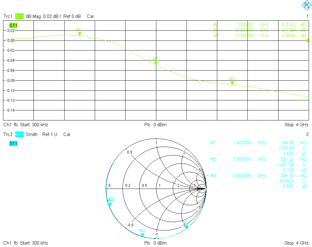
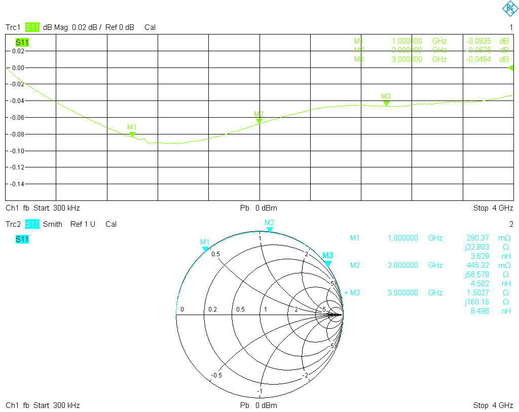
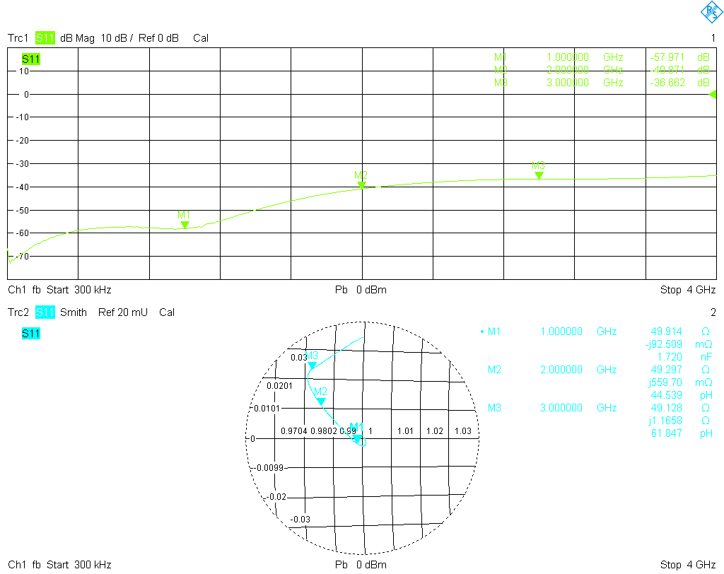
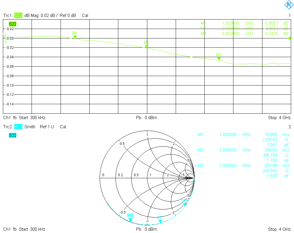
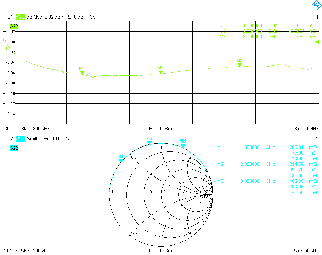
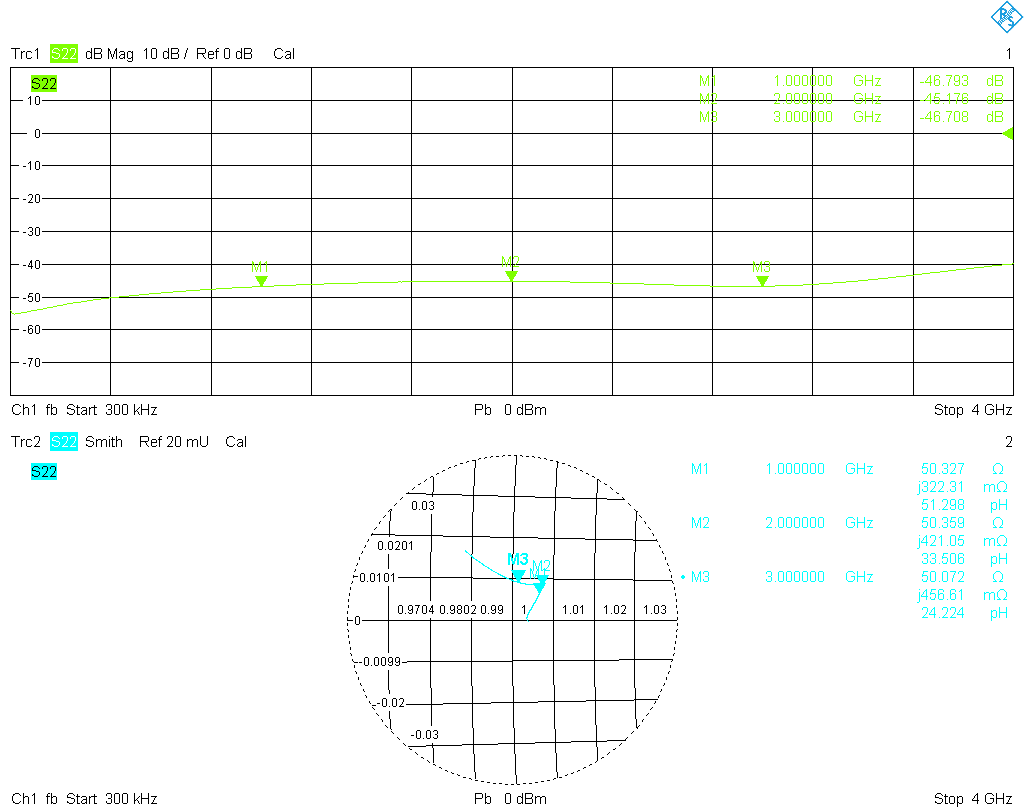
The open and short standards are somewhat lossy, but this is easily addressed by the common error correction models. The match standards are are a bigger problem; surely they are not shoddy and are certainly adequate as a general purpose termination, but are far from what one would expect from a calibration standard. The matches usually will set the limit on the accuracy of a cal kit even after correction with the coefficients method, since open and short are usually very precise after correction, but there is no general parametric model to adequately correct a match. It is interesting to note that between 1 GHz and 2 GHz the return loss of the female match worsens by about 20 dB and remains below only −35 dB, while the male match is much better and remains well below −45 dB almost up to 4 GHz. This despite the fact that the female standards are rated to a much higher frequency!
Another quality feature of a cal kit is the relative phase response of open and short over frequency. The error correction algorithm applied by the VNA is most stable (i.e., the error terms determined during calibration are least sensitive to variations in the measured reflection factors of the cal standards) if the responses of the open, short and match are spaced as far apart as possible on the Smith chart at every frequency in the band of interest. This is the case if, on the Smith chart, open, short and match are located on a straight line at every frequency, with the match at the center. In the extreme case, if open and short happen to rotate at very different rates around the outer edge of the Smith chart as frequency is increased, they will finally meet. At that frequency, they look alike (except perhaps for small differences in loss), and calibration fails. Thus the phase response of open and short should ideally be 180° apart. In the following two graphs the difference in the phase response of open and short (red trace) for the female kit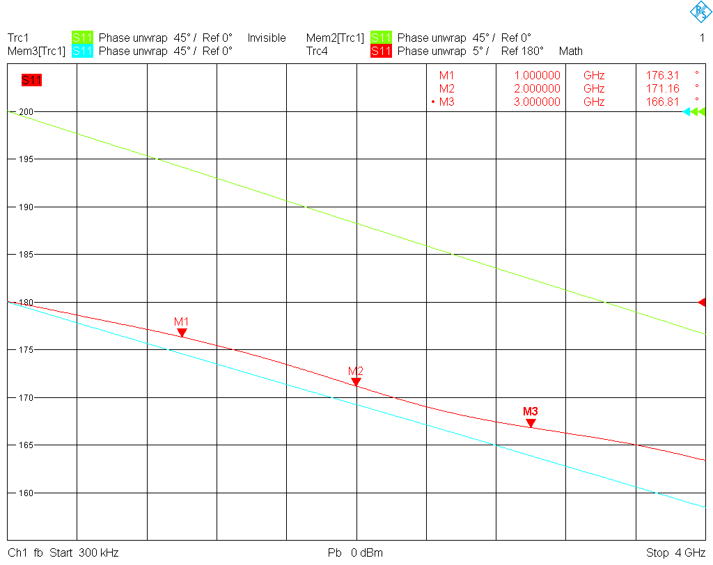 as well as for the male kit
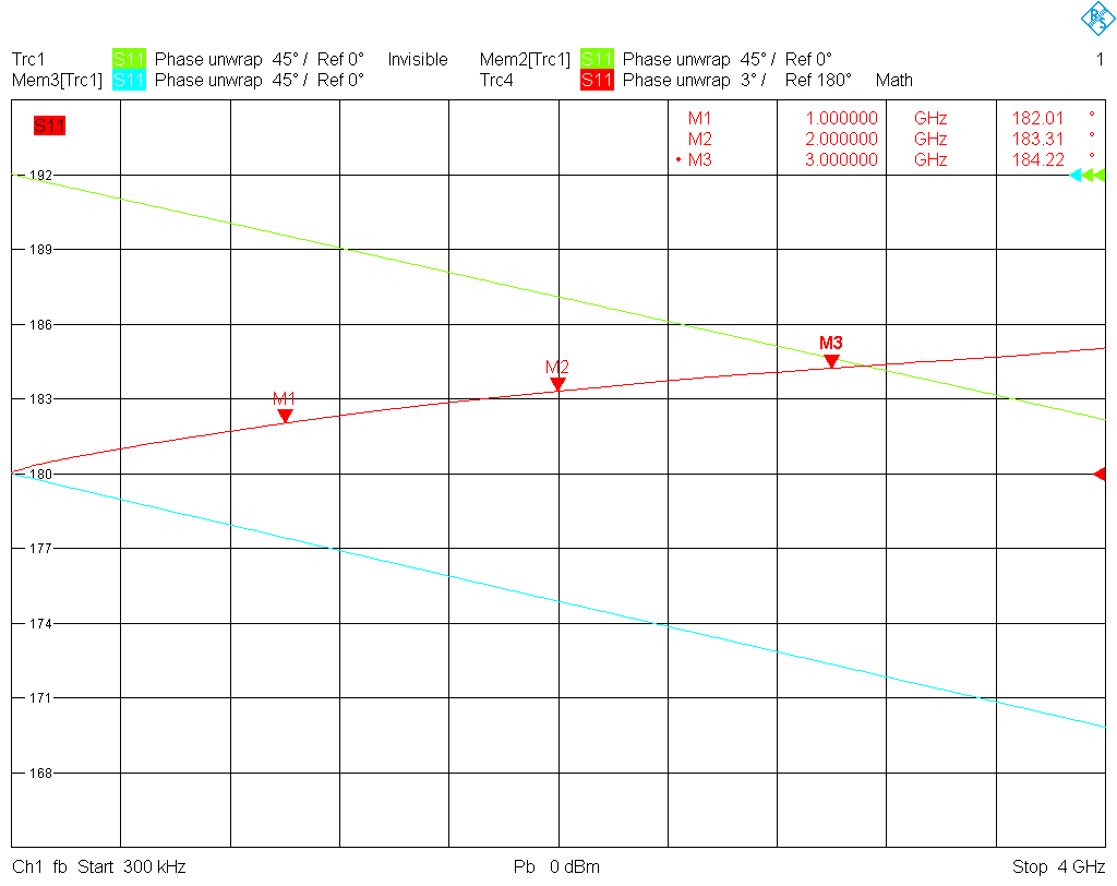 is plotted over frequency. For the female kit, the phase difference remains below 17°, and for the male kit below 6° in magnitude up to 4 GHz. This is actually a very good result.
Error correction: possibilities
There are two commonly used approaches to correct for the deviations of coaxial cal standards from ideal ones. The first uses a physical model of the cal standards, which is parametrized by a small set of numbers. This has the advantage of requiring only very little memory to store it, which was an important point in earlier VNAs, which used low density floppy disks and had limited instrument memory. Moreover, there is no hard upper frequency limit up to which the model can be evaluated. The drawback is, of course, that the cal standard has to follow the general model to a good degree. As mentioned before, for the match this is not easy (look at the Smith diagrams of the matches—it seems plausible that their reflection coefficient does not follow a simple model). The second approach is to use measured S11 data for the one-port standards and directly apply it for error correction in the VNA, possibly together with interpolation between the individual data points. This approach is model free, and ultimately its precision is only limited by the repeatability and stability of the cal standards and the accuracy of the measured data, but it can of course only be used up to the frequency for which correction data is available. Needless to say that today virtually all modern professional VNA support the use of S-parameter data for correction, even though some hobbyist's or ham radio kit don't.
The coefficients method
The one-port cal standards are modeled as follows: The port of the standard is connected to a TEM transmission line of a certain length, which is terminated by a frequency dependent impedance. This transmission line is exhaustively characterized by two parameters, namely its impedance and its complex propagation constant, which also includes losses. Besides these two quantities, the line length also has to be taken into account. There are various ways to parametrize the influence of the transmission line on the reflection coefficient of the cal standard at its port. We will follow the Keysight approach, which uses three parameters, called offset delay, offset impedance, and offset loss. Details can be found in the Keysight application note [4]. In most cases it is sufficient to assume that the offset impedance is equal to the system impedance (50 Ohms), and we shall make this assumption in the following.
The frequency dependent impedance terminating the transmission line is usually chosen to be given as a frequency dependent capacitance for the open standard, and a frequency dependent inductance for the short standard. Frequency dependence is described by a third order polynomial, i.e., the offset impedance is characterized by four coefficients for the open and short, respectively. Because of the difficulty to model the match, most professional cal kits use high precision matches with no correction data (more recently however even matches are corrected by measured S11 data, and have effectively superseded sliding loads, and also the modern electronic calibration modules rely on extensive correction data).
I have collected all relevant equations needed to fit the model parameters to the measured data in this pdf file. Currently no detailed derivation of the equations from first principles is provided in that document, but I plan to work out one and add it, as there seems to be a demand for an easy to understand derivation.
Fitting the model to measured data
After the model for the open and short cal standard has been described, we can go on to fit its parameters to the measured S-parameter data. To this end I have written a short script for GNU Octave, which can be downloaded here. The script also makes provisions to fit the match, only described by its resistance. Moreover, it can fit a thru, characterized by its delay time and offset loss, which needs of course the requisite S21 data. You can, of course, amend the script by a better model for the match (if you have one) or comment out the unnecessary parts. The script uses the Marquardt-Levenberg least squares algorithm from the optim package to solve the curve fitting problem. It also calculates a correlation coefficient from the residues after the curve fitting algorithm has terminated as a figure of merit of the fit.
After running the script on the Touchstone files I obtained the following coefficients for the open and short standards:
| Parameter | Male | Female |
|---|---|---|
| Offset delay in sec | 2.4034×10⁻¹¹ | 7.4010×10⁻¹¹ |
| Offset loss in Ohms/sec | 6.2590×10+09 | 4.3831×10+09 |
| C0 in F | 5.3424×10⁻¹³ | −3.1060×10⁻¹⁴ |
| C1 in F/Hz | 9.3381×10⁻²⁴ | 2.3250×10⁻²³ |
| C2 in F/Hz² | 6.1223×10⁻³⁴ | −8.8868×10⁻³³ |
| C3 in F/Hz³ | 9.8884×10−43 | 8.8375×10−43 |
| Parameter | Male | Female |
|---|---|---|
| Offset delay in sec | 2.7086×10⁻¹¹ | 2.8549×10⁻¹¹ |
| Offset loss in Ohms/sec | 6.3670×10+09 | 8.5102×10+09 |
| L0 in H | 1.3188×10−09 | 1.8993×10−09 |
| L1 in H/Hz | −2.5509×10⁻²² | 1.2329×10⁻¹⁹ |
| L2 in H/Hz² | 5.4689×10⁻³⁰ | −6.1382×10⁻²⁹ |
| L3 in H/Hz³ | 1.6595×10−39 | 2.3858×10−38 |
In the curve fitting done here all six parameters were unconstrained and treated with equal weights. For the intended purpose of the cal kit this approach is okay, but there may be reasons to proceed differently. Note that the parameters are not uniquely determined by the data. In fact, at a particular frequency, the phase delay can be caused by the offset delay (due to the offset length of the cal standard) or by the frequency dependent reactance. The frequency dependence of both contributions can be different in general, but the reactance's dependence can be adjusted quite arbitrarily by the third order polynomial, and hence can be used to compensate for the offset delay. This freedom is used in the coefficients for professional cal kits to optimize the high frequency behavior of the corrected kit. See page 177 of Dunsmore's book [1] for some remarks on this issue.
If you do not like to use Octave you may want to look at the METAS VNA Tools, available from the Swiss national metrological institute (METAS). That software offers a GUI approach to fitting calibration standard models to measured S-parameter data. The METAS VNA tools can handle parameters in the Keysight, Rohde & Schwarz and Anritsu formats.
Performance checks
To check the performance of the corrected cal kit, various devices can be measured on the calibrated VNA. Among them are airlines with a very precisely known impedance. Properly terminated they can provide a precise offset short or offset match, which is suitable to check the effective source match and directivity. If no precision airline is available, a piece of rigid coaxial line can be used instead. A full two-port calibration can be checked by measuring reference attenuators, airlines, or non-matched devices such as a Beatty standard, or by performing a T-check [5].
One-port checks
First let's do a one-port check by measuring an offset short. Since this is a highly reflective DUT the error term with dominant influence on the vector corrected measurement result will be the source port match, thus this test provides information about the effective source port match. By measuring an offset short, the residual port match error contribution will add or subtract, depending on phase relation (i.e., frequency), thereby yielding a ripple pattern superimposed on the S11 response of the line. The ripple amplitude provides information about the effective source port match.

The procedure is the following: After entering the correction coefficients into the VNA, port 1 is set up with a male and port 2 with a female connector. Then a full one-port calibration is performed on each port with the SMA kit; port 1 is calibrated with the female cal standards, and port 2 with the male standards. Next a very precise beadless airline with 3.5 mm inner diameter and 75 mm length (Maury Microwave model 8043S7.5) is connected to each of the ports; its opposite end is terminated with a short. For the male port (female cal standards) this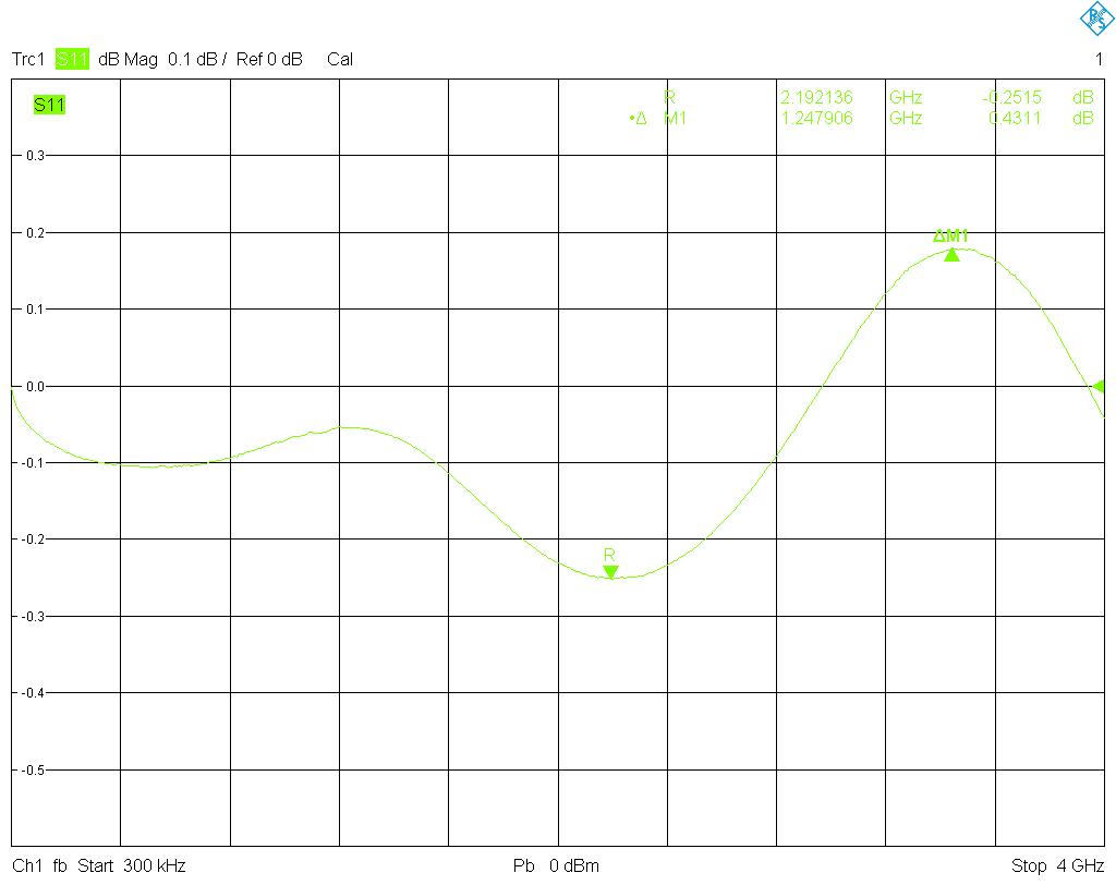 ripple pattern is obtained, and for the female port (male cal standards) this
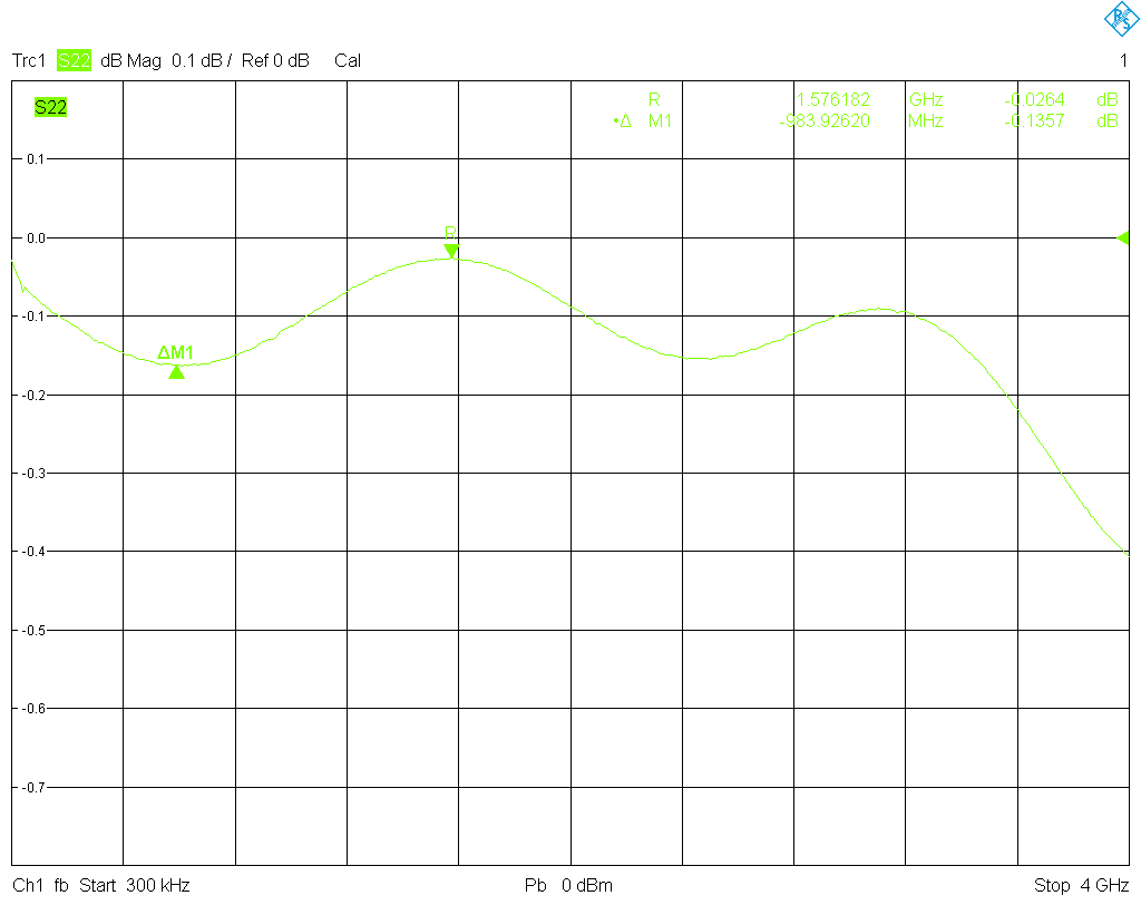 . For a maximum frequency of 4 GHz the airline is a bit short, with only two ripple periods over the entire frequency span, but still usable. Unfortunately I do not have a longer airline, just another 75 mm one; a series connection of them would require an adapter to support the center conductor.
It is seen that for both male and female cal standards the ripple amplitude is acceptable up to less than 2 GHz, and remains well below 0.2 dB. The male standards are well behaved to a somewhat higher frequency, whereas the ripple explodes from 2 GHz onward for the female standards, and rises to more than 0.4 dB. Since the major influencing factor for the quality of the calibration is the return loss of the match (provided nothing is fundamentally wrong with the open and the short—all three calibration standards contribute to the source port match error term), this was to be expected given the measured results for the matches. In particular, the worsening of the return loss of the female match is reflected in the ripple pattern.
Next let's measure an offset match. This is a highly absorbing DUT, thus the directivity error term will have a dominant influence on the vector corrected measurement result, and the resulting ripple pattern provides information about the effective directivity of the reflectometer. For the test the short at the end of the airline is replaced by a good quality male or female match (Hewlett-Packard model 909D and 909D Opt. 011, both are 3.5 mm precision coaxial terminations). It is important that this match has a larger return loss than the one used for calibration. For the male port (female cal standards) this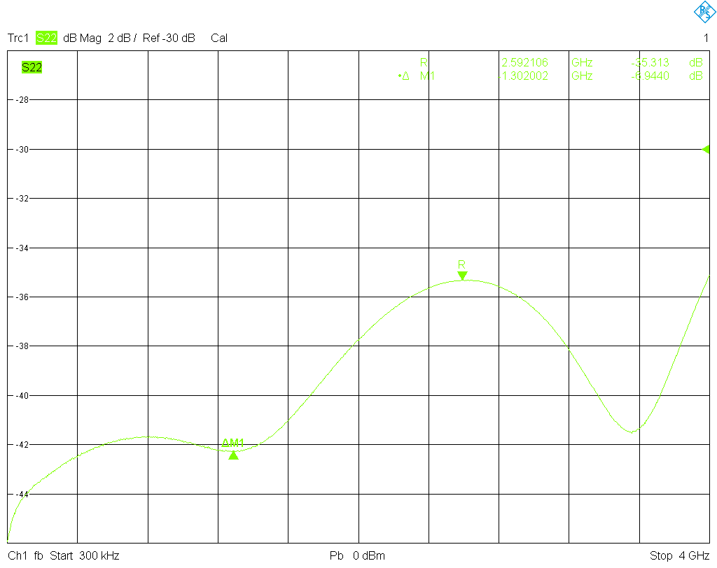 ripple pattern is obtained, and for the female port (male cal standards) this
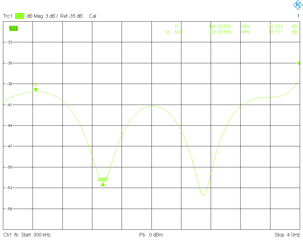 . Now looking at the mathematics behind the OSM calibration algorithm one can see that the directivity error term is equal to the S11 response of the match, provided it is assumed ideal (no correction data is used). Therefore, looking at the measured magnitudes of S11 for the male and female matches, it is no surprise that the ripple pattern is more equal over frequency for the male match standard, and that the ripple amplitude is smaller at low frequencies for the female match standard (look at the first ripple period), until it grows at higher frequencies.
Two-port checks
For a two-port check port 1 was configured with a male and port 2 with a female connector at the end of cables to facilitate connections to the verification standards. A full two-port calibration was performed using the SMA cal kit and the above correction data; the thru was flush (a UOSM calibration [8] was used, which is also known as unknown or reciprocal thru calibration). Here a non-negligible error is incurred by cable flexure because the cables used are not phase stable (too lazy to get out the proper test port cables).
First I measured a 3.5 mm reference attenuator with 20 dB nominal attenuation, which is part of the Hewlett-Packard 85053A verification kit, which I happen to have. The result can be seen here . That looks reasonably accurate with no signs of ripple.
Next a Maury model 8044S60 Beatty standard is measured. The Beatty standard, just like the T-check, has the virtue of checking the calibration for a non-matched DUT. It consists a 3.5 mm airline with a 25 Ohms section of 49.94 mm length. The result of a transmission and reflection measurement is seen here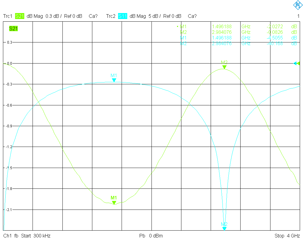 . Due to the two discontinuities of the transmission line the Beatty standard is reflective; only when the length of its 25 Ohms section becomes equal to half a wavelength (at 3 GHz), its reflection coefficient vanishes. When the length of the 25 Ohms section becomes equal to a quarter wavelength (at 1.5 GHz), its return loss is, in theory and neglecting losses, equal to approx. 4.44 dB. Here is an Octave script that calculates the S-matrix of an ideal Beatty standard (with the dimensions of the Maury device) and stores it as a Touchstone (s2p) file. Losses are neglected, as well as the fact that at the impedance step non-propagating TE and TM modes are excited, which store energy and act like a capacitor to ground at the discontinuity (see Marcuvitz's book [2] for details as well as an approximate expression for this capacity in a coaxial geometry, or Pozar's book [3] for an introduction to the general principles and an easy waveguide example).
As can be seen from the measured transmission and reflection data of the Beatty standard, it matches the theoretical expectations quite closely, except for some losses. There is some slight ripple on the transmission curve, which is probably due to the residual port match error, and hence due to the imperfections of the matches of the SMA cal kit (this ripple is not there when using the Maury cal kit). All in all nothing major seems to be wrong with this calibration for use in transmission measurements.
One could go on to measure more attenuators (the 85053A verification kit contains another 40 dB reference attenuator), or an airline between two ports and compare its phase response with theory, or check the reflection phase response of the Beatty standard, or perform a T-check, etc., but I decided to leave it well alone at this point as this is certainly not a precision cal kit.
Needless to say that with the direct use of the S-parameter data of the cal standards for correction, the calibration achieved is not much different from the Maury kit.


Some remarks on residual errors
Let's come back to the case of a single port and the problem of checking it using an offset short and the resulting ripple plot. The question arises which ripple amplitude is acceptable and how it is related to the residual errors of the calibration.
Consider a single VNA port for which error correction is applied, and which is connected to an impedance with reflection factor $\Gamma$. The influence of the residual errors on the measured wave quantities can be represented by the following signal flow graph.

Here $E_{\rm DF}$ is the residual directivity error, $E_{\rm SF}$ is the residual source match error, and $E_{\rm RF}$ is the residual reflection tracking error. Once again, these are the residual errors which remain after calibration, not the error terms that the analyzer applies to correct the measurement. Moreover, $S_{11}^{\rm m}=b_{\rm m}/a_{\rm m}$ is the measured S-parameter. From the signal flow graph, \begin{align} S_{11}^{\rm m}&=E_{\rm DF}+(1-E_{\rm RF})\frac{\Gamma}{1-E_{\rm SF}\Gamma}\\ &\approx E_{\rm DF}+(1-E_{\rm RF})\Gamma+(1-E_{\rm RF})E_{\rm SF}\Gamma^2. \end{align} The approximation is obtained by the first order Taylor expansion of $1/(1-E_{\rm SF}\Gamma)\approx1+E_{\rm SF}\Gamma$ at zero, which is accurate for $\lvert E_{\rm SF}\rvert\ll1$.
Consider a precision reflectionless airline (with $S_{11}=S_{22}=0$) of length $\ell$ and with transmission constant $\gamma=\alpha+\mathord{\rm i}\beta$, which is connected to the port, and has an ideal short at its opposite end. Then $\Gamma=-\mathord{\rm e}^{-2\gamma\ell}$, hence \[S_{11}^{\rm m}=-(1-E_{\rm RF})\mathord{\rm e}^{-2\gamma\ell}+E_{\rm DF}+(1-E_{\rm RF})E_{\rm SF}\mathord{\rm e}^{-4\gamma\ell}.\] In this expression the first term describes the influence of the shorted airline, impaired by the reflection tracking error; the second term is the directivity error, and the third term is due to the source match error.
We will give a simplified treatment that makes some assumptions. We can assume that the line is nearly lossless (i.e., $\alpha\approx0$). Moreover, assume that the residual reflection tracking error is small (which it usually is in practice), i.e., $E_{\rm RF}\approx0$. Thus \[S_{11}^{\rm m}=-\mathord{\rm e}^{-2\mathord{\rm i}\beta\ell}+E_{\rm DF}+E_{\rm SF}\mathord{\rm e}^{-4\mathord{\rm i}\beta\ell}.\]
It is seen from the first equation that when an ideal open or short is measured, and if for the open or short the residual errors are small (as can be assumed since the open and short standards are well corrected especially at low frequencies), i.e., $S_{11}^{\rm m}\approx\pm1$, it follows that $E_{\rm DF}\approx-E_{\rm SF}$. This implies \[S_{11}^{\rm m}=-\mathord{\rm e}^{-2\mathord{\rm i}\beta\ell}+E_{\rm SF}(1-\mathord{\rm e}^{-4\mathord{\rm i}\beta\ell}),\] and for the magnitude, \[\lvert S_{11}^m\rvert=\lvert1-E_{\rm SF}(\mathord{\rm e}^{2\mathord{\rm i}\beta\ell}-\mathord{\rm e}^{-2\mathord{\rm i}\beta\ell})\rvert=\lvert1-2E_{\rm SF}\cdot\sin(2\beta\ell)\rvert.\] Thus $\lvert S_{11}^{\rm m}\rvert$ shows a ripple pattern, and assuming that $E_{\rm SF}$ varies more slowly with frequency than $\sin(2\beta\ell)$, we find that the ripple has a peak-to-peak amplitude between \[\sqrt{1+4\lvert E_{\rm SF}\rvert^2}-1\approx2\lvert E_{\rm SF}\rvert^2\] and \[4\lvert E_{\rm SF}\rvert,\] depending on the phase of $E_{\rm SF}$. The ripple period is $c_0/2\ell$, which is approximately 2 GHz for the 75 mm airline used here.
This derivation with its simplifying assumptions is not the most sophisticated way to analyze a ripple test. It should be noted that in the case of a shorted airline the ripple includes contributions from all residual error terms. By a time domain analysis of the full ripple pattern described by the general equation above, more information about the individual residual error contributions can be extracted—see the literature, e.g., the paper by Wübbeler et. al. [6].
In fact, EURAMET [7] recommends a different estimate for the residual source match error than we derived above: For a shorted airline generating a peak-to-peak ripple $r$ in $\lvert S_{11}^{\rm m}\rvert$, the residual source match error is estimated as $r=2\lvert E_{\rm SF}\rvert$. Note that this is exactly the peak-to-peak ripple of the term $\lvert1+E_{\rm SF}\mathord{\rm e}^{-2\mathord{\rm i}\beta\ell}\rvert$ as $\beta$ varies (independent of the phase of $E_{\rm SF}$). This estimate lies between the two extreme cases that we found in our derivation, i.e., \[2\lvert E_{\rm SF}\rvert^2\leq2\lvert E_{\rm SF}\rvert\leq4\lvert E_{\rm SF}\rvert.\] In particular, it is seen that in some cases the residual port match error may be underestimated by using the EURAMET recommendation (it is worth noting that in section 1.2.2 the guideline explicitly warns about the uncertainties of the ripple method). Nevertheless, here we will follow the guideline in evaluating the ripple pattern.
Define now the effective source port match as $M=\lvert E_{\rm SF}\rvert$. Let $r=r^+-r^-$ be the the peak-to-peak ripple of $S_{11}^{\rm m}$, and $\Delta=L^+-L^-$ be the corresponding peak-to-peak ripple on the dB scale. Using the EURAMET recommendation, we then obtain for the effective source port match \begin{align} M({\rm dB})&=-20\cdot\log\bigl(\tfrac12(r^+-r^-)\bigr)\\ &=-20\cdot\log\bigl(\tfrac1210^{L^+/20}-\tfrac1210^{L^-/20}\bigr). \end{align} For small ripple amplitude and $\lvert S_{11}^{\rm m}\rvert$ close to $1$ we can write $M\approx1-10^{-\Delta/40}$, and thus \[M({\rm dB})\approx-20\cdot\log\bigl(1-10^{-\Delta/40}\bigr).\]
As mentioned above, for a terminated airline the ripple yields information about residual directivity. According to EURAMET, if $r$ is the peak-to-peak ripple of an airline terminated with a good quality match, the residual directivity error can by estimated from $r=2\lvert E_{\rm DF}\rvert$. This can be justified by a similar derivation as shown above.
For some more remarks on calibration, verification, and the ripple test see the EURAMET VNA calibration guide [7].
Coming back to the measurement of the shorted airline, we found a ripple of less than 0.15 dB up to about 2 GHz with the shorted airline. This translates to a source port match of about 40 dB. Moreover, from the measurement of the airline terminated with a match we obtain a residual directivity of approximately 0.005 for the female kit and 0.004 for the male kit, both in excess of 45 dB. This is an acceptable value for a casual cal kit.
Bibliography
- Dunsmore, J.P.: Handbook of Mircowave Component Measurements. Chichester: Wiley (2012).
- Marcuvitz, N.: Waveguide Handbook. New York: McGraw-Hill (1951).
- Pozar, D.M.: Microwave Engineering. 4th Ed. New York: Wiley (2012).
- Keysight Technologies: Specifying Calibration Standards and Kits for Keysight Vector Network Analyzers. Keysight Application Note 5989-4840EN.
- Ostwald, O.: T-Check Accuracy Test for Vector Network Analyzers utilizing a Tee-junction. Rohde & Schwarz Application Note 1EZ43_0E.
- Wübbeler, G., Elster, C., Reichel, T., Judaschke, R.: Determination of the complex residual error parameters of a calibrated one-port vector network analyzer. IEEE Trans. Instr. Meas. 58, 3238–3244 (2009).
- EURAMET: Guidelines on the Evaluation of Vector Network Analysers (VNA). EURAMET Calibration Guide No. 12.
- Ferrero, A., Pisani, U.: Two-port network analyzer calibration using an unknown 'thru'. IEEE Microwave Guided Wave Lett. 2, 505–507 (1992).